Chuanshuoge: 2019

Tuesday 31 December 2019

django mpld3 live stock plot

server starts

1 minute elapsed

5 minute passed

#power shell

pip install yahoo-fin
pip install requests_html

------------------------------------
#django/app/view

from django.shortcuts import render
import matplotlib.pyplot as plt
from mpld3 import plugins, fig_to_html, save_html, fig_to_dict
import json
import numpy as np
from datetime import datetime
from yahoo_fin import stock_info as si

class NumpyEncoder(json.JSONEncoder):
def default(self, obj):
if isinstance(obj, np.ndarray):
return obj.tolist()
return json.JSONEncoder.default(self, obj)

x, y = [], []

def index(request):
fig1, ax1 = plt.subplots()
global x, y

x.append(datetime.now())
price = si.get_live_price('aapl')
y.append(price)

if len(x) < 2:
return render(request, 'mpld/index.html')

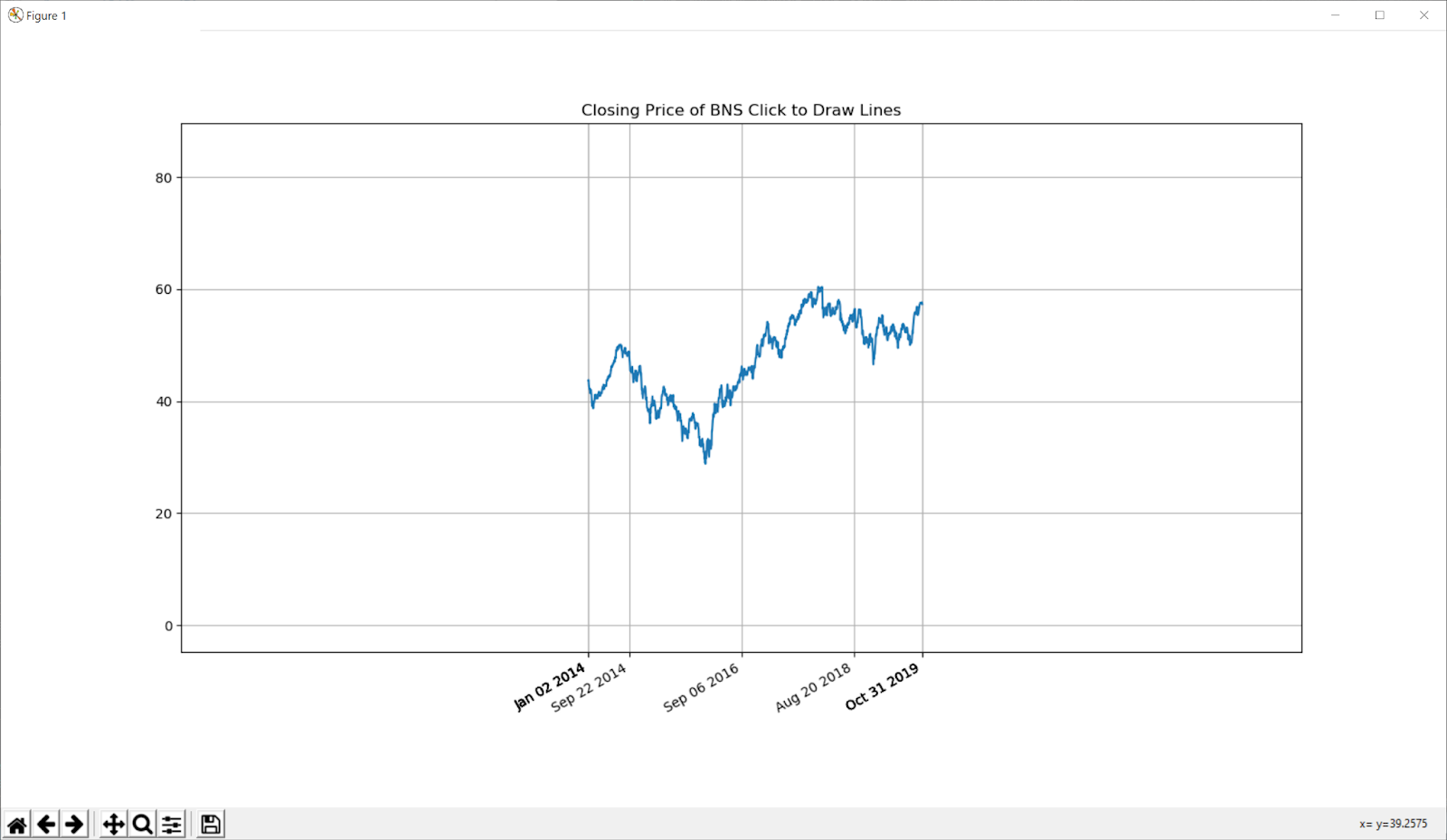
ax1.plot(x, y)
ax1.grid(color='lightgray', alpha=0.7)
ax1.set_xlabel('time', fontsize=15)
ax1.set_ylabel('price', fontsize=15)
ax1.set_title('Live Apple stock Price', fontsize=20)

g1 = json.dumps(fig_to_dict(fig1), cls=NumpyEncoder)

return render(request, 'mpld/index.html',
{'graph1': g1})

-----------------------------------

#django/template/index

<!DOCTYPE html>

<head>

</head>

<body>

<div id="fig1">graph1</div>

</div>

mpld3.draw_figure("fig1", {{graph1 | safe}});

</script>

</body>

</html>

reference:
https://stackoverflow.com/questions/441147/how-to-subtract-a-day-from-a-date
http://theautomatic.net/2018/07/31/how-to-get-live-stock-prices-with-python/
http://chuanshuoge2.blogspot.com/2019/12/django-mpld3-multiple-plots-on-html-page.html

auto refresh page
https://stackoverflow.com/questions/2787679/how-to-reload-page-every-5-seconds

yahoo_fin
http://theautomatic.net/yahoo_fin-documentation/

Monday 30 December 2019

Naked Science

https://www.youtube.com/user/PioneerProductionsUK/videos

django mpld3 multiple plots on a html page

#mpld/views

from django.http import HttpResponse
from django.shortcuts import render
import matplotlib.pyplot as plt
from mpld3 import plugins, fig_to_html, save_html, fig_to_dict
import json
import numpy as np

#for numpy array is not json serializable error
class NumpyEncoder(json.JSONEncoder):
def default(self, obj):
if isinstance(obj, np.ndarray):
return obj.tolist()
return json.JSONEncoder.default(self, obj)

def index(request):
fig1, ax1 = plt.subplots()
np.random.seed(0)
x1, y1 = np.random.normal(size=(2, 200))
color, size = np.random.random((2, 200))

ax1.scatter(x1, y1, c=color, s=500 * size, alpha=0.3)
ax1.grid(color='lightgray', alpha=0.7)

fig2, ax2 = plt.subplots(3, 3, figsize=(6, 6))
fig2.subplots_adjust(hspace=0.1, wspace=0.1)
ax2 = ax2[::-1]

X2 = np.random.normal(size=(3, 100))
for i in range(3):
for j in range(3):
ax2[i, j].xaxis.set_major_formatter(plt.NullFormatter())
ax2[i, j].yaxis.set_major_formatter(plt.NullFormatter())
points = ax2[i, j].scatter(X2[j], X2[i])

plugins.connect(fig2, plugins.LinkedBrush(points))

fig3, ax3 = plt.subplots()
x3 = np.linspace(-5, 15, 1000)
for offset in np.linspace(0, 3, 4):
ax3.plot(x3, 0.9 * np.sin(x3 - offset), lw=5, alpha=0.4,
label="Offset: {0}".format(offset))
ax3.set_xlim(0, 10)
ax3.set_ylim(-1.2, 1.0)
ax3.text(5, -1.1, "Here are some curves", size=18, ha='center')
ax3.grid(color='lightgray', alpha=0.7)
ax3.legend()

fig4, ax4 = plt.subplots(2, 2, figsize=(8, 6), sharex='col', sharey='row')
fig4.subplots_adjust(hspace=0.3)

np.random.seed(0)

for axi in ax4.flat:
color = np.random.random(3)
axi.plot(np.random.random(30), lw=2, c=color)
axi.set_title("RGB = ({0:.2f}, {1:.2f}, {2:.2f})".format(*color),
size=14)
axi.grid(color='lightgray', alpha=0.7)

#save_html(fig, 'fig.html')
g1 = json.dumps(fig_to_dict(fig1), cls=NumpyEncoder)
g2 = json.dumps(fig_to_dict(fig2), cls=NumpyEncoder)
g3 = json.dumps(fig_to_dict(fig3))
g4 = json.dumps(fig_to_dict(fig4))

return render(request, 'mpld/index.html',
{'graph1': g1,
'graph2': g2,
'graph3': g3,
'graph4': g4})

--------------------------------

#mpld/templates/index.html

<!DOCTYPE html>

<head>

</head>

<body>

<div id="fig1">graph1</div>

</div>

<div id="fig2">graph2</div>

</div>

<div id="fig3">graph3</div>

</div>

<div id="fig4">graph4</div>

</div>

mpld3.draw_figure("fig1", {{graph1 | safe}});

mpld3.draw_figure("fig2", {{graph2 | safe}});

mpld3.draw_figure("fig3", {{graph3 | safe}});

mpld3.draw_figure("fig4", {{graph4 | safe}});

</script>

</body>

</html>

-----------------------------
#django_mpld3/settings

TEMPLATES = [
{
'DIRS': [os.path.join(BASE_DIR, 'mpld' , 'templates')],
...
},
]

reference:
https://github.com/mpld3/mpld3/issues/128
https://stackoverflow.com/questions/22981359/display-multiple-mpld3-exports-on-a-single-html-page/
https://stackoverflow.com/questions/31151229/django-passing-json-from-view-to-template
https://stackoverflow.com/questions/26646362/numpy-array-is-not-json-serializable
https://mpld3.github.io/notebooks/mpld3_demo.html

5 Python Libraries for Creating Interactive Plots

https://mode.com/blog/python-interactive-plot-libraries

Sunday 29 December 2019

django mpld3 point tooltip

hover on point, tooltip with x, y position is displayed

from django.http import HttpResponse

import matplotlib.pyplot as plt

from mpld3 import plugins, fig_to_html, save_html

def index(request):

fig, ax = plt.subplots()

points = ax.plot(range(10), 'o')

plugins.connect(fig, plugins.PointLabelTooltip(points[0]))

save_html(fig, 'fig.html')

g = fig_to_html(fig)

return HttpResponse(g)

figure is also saved as html file

double click on saved file, browser will open it up

reference:

https://mpld3.github.io/modules/API.html#module-mpld3.plugins

http://chuanshuoge2.blogspot.com/2019/12/django-mpld3-1.html

django mpld3 1

mpld3 - bringing matplotlib to browser

The mpld3 project brings together Matplotlib, the popular Python-based graphing library, and D3js, the popular JavaScript library for creating interactive data visualizations for the web. The result is a simple API for exporting your matplotlib graphics to HTML code which can be used within the browser, within standard web pages, blogs, or tools such as the IPython notebook.

#powershell

pip install mpld3
pip install Jinja2

-----------------------
#mpld/views

from django.http import HttpResponse
import matplotlib.pyplot as plt, mpld3

def index(request):
fig = plt.figure()
plt.plot([1, 2, 3, 4])
g = mpld3.fig_to_html(fig)
return HttpResponse(g)

reference:
https://mpld3.github.io/
https://stackoverflow.com/questions/18944345/importerror-no-module-named-jinja2/18983050
https://stackoverflow.com/questions/24127938/using-mpld3-to-add-graphs-into-django-projects

Saturday 28 December 2019

django matplotlib response as png

#matplot/views

from django.http import HttpResponse
import matplotlib.pyplot as plt
import numpy as np
import io

def index(request):
return HttpResponse('<h1>matplotlib app homepage</h1>')

def plot(request):
# Data for plotting
t = np.arange(0.0, 2.0, 0.01)
s = 1 + np.sin(2 * np.pi * t)

fig, ax = plt.subplots()
ax.plot(t, s)
ax.set(xlabel='time (s)', ylabel='voltage (mV)',
title='About as simple as it gets, folks')
ax.grid()

buf = io.BytesIO()
plt.savefig(buf, format='png')
plt.close(fig)

response = HttpResponse(buf.getvalue(), content_type='image/png')
return response

--------------------------------
#matplot/urls

from django.urls import path
from . import views

urlpatterns = [
path('', views.index, name='index'),
path('chart/', views.plot, name='chart')
]

------------------------------
#django_matplotlib/urls

from django.contrib import admin
from django.urls import path, include

urlpatterns = [
path('admin/', admin.site.urls),
path('matplot/', include('matplot.urls')),
]

reference:
https://stackoverflow.com/questions/49542459/error-in-django-when-using-matplotlib-examples
https://stackoverflow.com/questions/40534715/how-to-embed-matplotlib-graph-in-django-webpage

Friday 27 December 2019

matplotlib mouse scroll event zoom

original graph year 2014 - 2019

scroll mouse to zoom in year 2016 - 2019

xaxis date updates with zoom

scroll to zoom out, xaxis is collapsed

zoom in again, xaxis expands again

from matplotlib import pyplot as plt
import numpy as np
import datetime as dt
import pandas_datareader.data as web

class ZoomClass(object):
def __init__(self, base_scale, tick_num, x, y):
self.base_scale = base_scale
self.tick_num = tick_num
self.x = x
self.y = y

def zoom_event(self, event):
if not event.inaxes:
return
# get the current x and y limits
cur_xlim = ax.get_xlim()
cur_ylim = ax.get_ylim()

xdata = event.xdata # get event x location
ydata = event.ydata # get event y location

if event.button == 'up':
# zoom in
scale_factor = self.base_scale
elif event.button == 'down':
# zoom out
scale_factor = 1 / self.base_scale
else:
scale_factor = 1
print(event.button)

# set new boundary, center is mouse position
ax.set_xlim([xdata - (xdata-cur_xlim[0]) / scale_factor, xdata + (cur_xlim[1]-xdata) / scale_factor])
ax.set_ylim([ydata - (ydata-cur_ylim[0]) / scale_factor, ydata + (cur_ylim[1]-ydata) / scale_factor])
# get the current x limits again
cur_xlim = ax.get_xlim()
#update xaxis date range, numbers on axis updates automatically, dates need update manually
xticks = []
for i in range(0, self.tick_num):
value = int(cur_xlim[0]) + int(i * (cur_xlim[1] - cur_xlim[0]) / self.tick_num)
# take care of values beyond x limits
if value < 0:
value = 0
if value > np.max(self.x):
value = np.max(self.x)
xticks.append(value)
print(xticks)

xlabels = [x_format[xticks[i]] for i in range(0, self.tick_num)]
ax.set_xticks(xticks)
ax.set_xticklabels(xlabels)
# refresh plot
fig.canvas.draw()

start = dt.datetime(2014, 1, 1)
end = dt.datetime(2019, 10, 30)
ticker = 'BNS'

df = web.DataReader(ticker, 'yahoo', start, end)
x = df['Adj Close'].index
y = df['Adj Close'].values
#number index is need for the cursor position, xaxis is mapped with integer first and converted to date later
x_num_index = np.arange(0, len(x), 1)

fig, ax = plt.subplots()
plot1 = ax.plot(x_num_index, y)

#get default # of lables on x axis
n = len(ax.get_xticklabels())
print(n)

zoom_view = ZoomClass(1.2, n, x_num_index, y)
fig.canvas.mpl_connect('scroll_event', zoom_view.zoom_event)

x_format = x.strftime('%b %d %Y')
xticks = [int(i*len(x)/n) for i in range(0, n)]
xlabels = [x_format[int(i*len(x)/n)] for i in range(0, n)]
ax.set_xticks(xticks)
ax.set_xticklabels(xlabels)

ax.set_ylim([np.min(y), np.max(y)])
ax.set_title('Closing Price of %s Click to Draw Lines' %(ticker))

plt.gcf().autofmt_xdate()
plt.grid(True)
plt.show()

---------------------------------
#logs

up
[14, 148, 283, 417, 552, 686, 821, 955, 1090, 1225]
down
[0, 88, 250, 411, 573, 734, 896, 1057, 1219, 1380]
down
[0, 56, 250, 444, 638, 832, 1025, 1219, 1413, 1468]
up
[0, 154, 316, 477, 639, 800, 962, 1123, 1285, 1446]
up
[157, 291, 426, 560, 695, 830, 964, 1099, 1233, 1368]
up
[264, 376, 488, 600, 712, 824, 937, 1049, 1161, 1273]
up
[353, 446, 540, 633, 727, 820, 914, 1007, 1101, 1194]
up
[427, 505, 583, 661, 739, 817, 895, 973, 1051, 1129]
down
[324, 417, 511, 605, 698, 792, 886, 980, 1073, 1167]
down
[201, 313, 426, 538, 651, 763, 876, 989, 1101, 1214]
down
[53, 188, 323, 458, 593, 728, 863, 998, 1134, 1269]
up
[200, 312, 425, 538, 650, 763, 876, 988, 1101, 1214]
down
[26, 161, 296, 431, 567, 702, 837, 972, 1108, 1243]
...
up
[545, 639, 734, 828, 923, 1018, 1112, 1207, 1301, 1396]
up
[613, 691, 770, 849, 928, 1007, 1086, 1165, 1244, 1323]
up
[670, 735, 801, 867, 933, 999, 1065, 1130, 1196, 1262]
down
[612, 691, 770, 849, 928, 1007, 1086, 1165, 1244, 1323]
down
[542, 636, 731, 826, 921, 1016, 1111, 1206, 1301, 1396]
down
[500, 614, 728, 842, 956, 1070, 1184, 1298, 1412, 1468]
up
[573, 668, 763, 858, 953, 1048, 1143, 1238, 1333, 1428]
up
[637, 716, 795, 874, 953, 1033, 1112, 1191, 1270, 1349]
down
[572, 667, 762, 857, 952, 1047, 1142, 1238, 1333, 1428]
up
[666, 745, 824, 903, 983, 1062, 1141, 1221, 1300, 1379]
down
[566, 661, 756, 851, 947, 1042, 1137, 1232, 1328, 1423]
down
[446, 560, 674, 789, 903, 1018, 1132, 1246, 1361, 1468]
down
[286, 423, 560, 698, 835, 973, 1110, 1247, 1385, 1468]
down
[94, 258, 423, 588, 753, 918, 1083, 1248, 1413, 1468]
down
[0, 61, 259, 457, 655, 853, 1051, 1249, 1447, 1468]
down
[0, 0, 62, 300, 537, 775, 1012, 1250, 1468, 1468]
down
[0, 0, 0, 192, 477, 762, 1047, 1332, 1468, 1468]
down
[0, 0, 0, 60, 402, 744, 1086, 1428, 1468, 1468]
down
[0, 0, 0, 0, 312, 722, 1133, 1468, 1468, 1468]
down
[0, 0, 0, 0, 181, 674, 1166, 1468, 1468, 1468]
up
[0, 0, 0, 0, 289, 699, 1110, 1468, 1468, 1468]
up
[0, 0, 0, 35, 377, 719, 1061, 1403, 1468, 1468]
up
[0, 0, 0, 166, 451, 736, 1021, 1306, 1468, 1468]
up
[0, 0, 37, 275, 512, 750, 987, 1225, 1462, 1468]
up
[0, 0, 168, 366, 564, 762, 960, 1158, 1356, 1468]
up
[0, 97, 262, 427, 592, 757, 922, 1087, 1252, 1417]
down
[0, 0, 154, 352, 550, 748, 946, 1144, 1342, 1468]
up
[0, 84, 249, 414, 579, 744, 909, 1074, 1239, 1404]

reference:
https://stackoverflow.com/questions/11551049/matplotlib-plot-zooming-with-scroll-wheel
https://stackoverflow.com/questions/26131607/matplotlib-get-ylim-values
https://matplotlib.org/3.1.1/gallery/showcase/integral.html#sphx-glr-gallery-showcase-integral-py

Thursday 26 December 2019

那些令人难忘的BOSS战

Wednesday 25 December 2019

matplotlib mouse click event draw line

left click to set 1 point of a line, the second point follows the mouse position,

line is floating

left click again to complete the line

left click again to start a new line, line is floating

left click again to complete second line

draw third line

right click to delete 3rd line end point, line is floating

left click to set end point of 3rd line again, line is fixed

right click twice to delete 3rd line

delete second line

keep right click, original graph is intact

from matplotlib import pyplot as plt
import numpy as np
import datetime as dt
import pandas_datareader.data as web

class LineBuilder(object):
def __init__(self, fig, ax):
self.xs = []
self.ys = []
self.ax = ax
self.fig = fig

def mouse_click(self, event):
print('click', event)
if not event.inaxes:
return
#left click
if event.button == 1:
self.xs.append(event.xdata)
self.ys.append(event.ydata)
#add a line to plot if it has 2 points
if len(self.xs) % 2 == 0:
line, = self.ax.plot([self.xs[-2], self.xs[-1]], [self.ys[-2], self.ys[-1]], 'r')
line.figure.canvas.draw()

#right click
if event.button == 3:
if len(self.xs) > 0:
self.xs.pop()
self.ys.pop()
#delete last line drawn if the line is missing a point,
#never delete the original stock plot
if len(self.xs) % 2 == 1 and len(self.ax.lines) > 1:
self.ax.lines.pop()
#refresh plot
self.fig.canvas.draw()

def mouse_move(self, event):
if not event.inaxes:
return
#dtaw a temporary line from a single point to the mouse position
#delete the temporary line when mouse move to another position
if len(self.xs) % 2 == 1:
line, =self.ax.plot([self.xs[-1], event.xdata], [self.ys[-1], event.ydata], 'r')
line.figure.canvas.draw()
self.ax.lines.pop()

start = dt.datetime(2014, 1, 1)
end = dt.datetime(2019, 10, 30)
ticker = 'BNS'

df = web.DataReader(ticker, 'yahoo', start, end)
x = df['Adj Close'].index
y = df['Adj Close'].values
#number index is need for the cursor position, xaxis is mapped with integer first and converted to date later
x_num_index = np.arange(0, len(x), 1)

fig, ax = plt.subplots()
ax.plot(x_num_index, y)

draw_line = LineBuilder(fig, ax)
fig.canvas.mpl_connect('button_press_event', draw_line.mouse_click)
fig.canvas.mpl_connect('motion_notify_event', draw_line.mouse_move)

#get default # of lables on x axis
n = len(ax.get_xticklabels())
print(n)

x_format = x.strftime('%b %d %Y')
xlabels = [x_format[int(i*len(x)/n)] for i in range(0, n)]
ax.set_xticklabels(xlabels)

ax.set_ylim([np.min(y), np.max(y)])
ax.set_title('Closing Price of %s Click to Draw Lines' %(ticker))

plt.gcf().autofmt_xdate()
plt.show()

---------------------------------------
#logs

click button_press_event: xy=(243, 448) xydata=(129.8095001772421, 49.733963975081586) button=1 dblclick=False inaxes=AxesSubplot(0.125,0.2;0.775x0.68)
click button_press_event: xy=(447, 161) xydata=(522.8799401263872, 30.376382342657486) button=1 dblclick=False inaxes=AxesSubplot(0.125,0.2;0.775x0.68)
click button_press_event: xy=(700, 599) xydata=(1009.1782920476983, 59.91861493848242) button=1 dblclick=False inaxes=AxesSubplot(0.125,0.2;0.775x0.68)
click button_press_event: xy=(447, 234) xydata=(529.4506930074507, 35.30008777529497) button=1 dblclick=False inaxes=AxesSubplot(0.125,0.2;0.775x0.68)
click button_press_event: xy=(720, 549) xydata=(1060.785741080495, 56.54621395722387) button=1 dblclick=False inaxes=AxesSubplot(0.125,0.2;0.775x0.68)
click button_press_event: xy=(924, 480) xydata=(1457.8273154647482, 51.892300603087065) button=1 dblclick=False inaxes=AxesSubplot(0.125,0.2;0.775x0.68)
click button_press_event: xy=(837, 426) xydata=(1288.5007616832286, 48.25010754332782) button=3 dblclick=False inaxes=AxesSubplot(0.125,0.2;0.775x0.68)
click button_press_event: xy=(856, 520) xydata=(1566.6027451122914, 54.59022138809391) button=1 dblclick=False inaxes=AxesSubplot(0.125,0.2;0.775x0.68)
click button_press_event: xy=(756, 495) xydata=(1336.569036952411, 52.904020897464626) button=3 dblclick=False inaxes=AxesSubplot(0.125,0.2;0.775x0.68)
click button_press_event: xy=(610, 494) xydata=(1000.7198230389853, 52.83657287783946) button=3 dblclick=False inaxes=AxesSubplot(0.125,0.2;0.775x0.68)
click button_press_event: xy=(611, 249) xydata=(1003.0201601205841, 36.31180806967254) button=3 dblclick=False inaxes=AxesSubplot(0.125,0.2;0.775x0.68)
click button_press_event: xy=(611, 249) xydata=(1003.0201601205841, 36.31180806967254) button=3 dblclick=True inaxes=AxesSubplot(0.125,0.2;0.775x0.68)
click button_press_event: xy=(670, 446) xydata=(1138.7400479349135, 49.59906793583124) button=3 dblclick=False inaxes=AxesSubplot(0.125,0.2;0.775x0.68)
click button_press_event: xy=(650, 438) xydata=(1092.7333063029378, 49.05948377882987) button=3 dblclick=False inaxes=AxesSubplot(0.125,0.2;0.775x0.68)
click button_press_event: xy=(651, 438) xydata=(1095.0336433845364, 49.05948377882987) button=3 dblclick=False inaxes=AxesSubplot(0.125,0.2;0.775x0.68)

reference:
https://stackoverflow.com/questions/33569626/matplotlib-responding-to-click-events
http://chuanshuoge2.blogspot.com/2019/12/matplotlib-cursor.html
https://matplotlib.org/3.1.1/users/event_handling.html
https://stackoverflow.com/questions/4981815/how-to-remove-lines-in-a-matplotlib-plot
https://stackoverflow.com/questions/4098131/how-to-update-a-plot-in-matplotlib

Monday 23 December 2019

matplotlib mouse move event cursor

values display at upper left

cursor response to mouse move, cursor center always snaps to the plot

import matplotlib.pyplot as plt
import numpy as np
import datetime as dt
import pandas_datareader.data as web

class SnaptoCursor(object):
"""
Like Cursor but the crosshair snaps to the nearest x, y point.
For simplicity, this assumes that *x* is sorted.
"""

def __init__(self, ax, x, y, numberIndex):
self.ax = ax
self.lx = ax.axhline(color='r') # the horiz line
self.ly = ax.axvline(color='r') # the vert line
self.x = x
self.y = y
self.nIndex = numberIndex
# text location in axes coords
self.txt = ax.text(0.05, 0.9, '', transform=ax.transAxes)

def mouse_move(self, event):
if not event.inaxes:
return

x, y = event.xdata, event.ydata
indx = min(np.searchsorted(self.nIndex, x), len(self.x) - 1)
x = self.x[indx]
y = self.y[indx]
# update the line positions
self.lx.set_ydata(y)
self.ly.set_xdata(indx)

self.txt.set_text('x=%s\ny=%1.2f' % (x.strftime('%b %d %Y'), y))
self.ax.figure.canvas.draw()

start = dt.datetime(2014, 1, 1)
end = dt.datetime(2019, 10, 30)
ticker = 'BNS'

df = web.DataReader(ticker, 'yahoo', start, end)
print(df[:5])
print(df['Adj Close'].values[:5])
print(df['Adj Close'].index[:5])

x = df['Adj Close'].index
y = df['Adj Close'].values
#number index is need for the cursor position, xaxis is mapped with integer first and converted to date later
x_num_index = np.arange(0, len(x), 1)

fig, ax = plt.subplots()
ax.plot(x_num_index, y)
snap_cursor = SnaptoCursor(ax, x, y, x_num_index)
fig.canvas.mpl_connect('motion_notify_event', snap_cursor.mouse_move)

#get default # of lables on x axis
n = len(ax.get_xticklabels())
print(n)

x_format = x.strftime('%b %d %Y')
xlabels = [x_format[int(i*len(x)/n)] for i in range(0, n)]
print(xlabels)
ax.set_xticklabels(xlabels)

ax.set_ylim([np.min(y), np.max(y)])
ax.set_title('Closing Price of %s' %(ticker))

plt.gcf().autofmt_xdate()
plt.show()

----------------------------
#logs
High Low Open Close Volume Adj Close
Date
2014-01-02 62.750000 61.939999 62.549999 61.980000 425800.0 43.690678
2014-01-03 61.689999 61.060001 61.490002 61.500000 351100.0 43.790367
2014-01-06 61.360001 60.480000 61.340000 60.750000 427300.0 43.256340
2014-01-07 60.820000 59.869999 60.610001 59.889999 547600.0 42.643982
2014-01-08 59.840000 59.330002 59.770000 59.630001 540700.0 42.458855
[43.69067764 43.79036713 43.25634003 42.64398193 42.45885468]
DatetimeIndex(['2014-01-02', '2014-01-03', '2014-01-06', '2014-01-07',
'2014-01-08'],
dtype='datetime64[ns]', name='Date', freq=None)
10
['Jan 02 2014', 'Aug 01 2014', 'Mar 04 2015', 'Oct 01 2015', 'May 03 2016', 'Nov 30 2016', 'Jul 03 2017', 'Feb 01 2018', 'Aug 31 2018', 'Apr 04 2019']

reference:
http://chuanshuoge2.blogspot.com/2019/10/python-programming-for-finance-1.html
https://stackabuse.com/how-to-format-dates-in-python/
https://matplotlib.org/3.1.0/gallery/misc/cursor_demo_sgskip.html
https://stackoverflow.com/questions/11244514/modify-tick-label-text

matplotlib growing coil

import matplotlib.pyplot as plt
import matplotlib.animation as animation
import numpy as np

plt.style.use('dark_background')

fig = plt.figure()
ax = plt.axes(xlim=(-50, 50), ylim=(-50, 50))
#set line width
line, = ax.plot([], [], lw=2)

# initialization function
def init():
# creating an empty plot/frame
line.set_data([], [])
return line,

# lists to store x and y axis points
xdata, ydata = [], []

# animation function
def animate(i):
# t is a parameter
t = 0.1 * i

# x, y values to be plotted
x = t * np.sin(t)
y = t * np.cos(t)

# appending new points to x, y axes points list
xdata.append(x)
ydata.append(y)
line.set_data(xdata, ydata)
return line,

plt.title('Creating a growing coil with matplotlib!')
# hiding the axis details
plt.axis('off')

anim = animation.FuncAnimation(fig, animate, init_func=init,
frames=500, interval=10, blit=True)

anim.save('coil.gif', fps=50)

reference:
https://towardsdatascience.com/animations-with-matplotlib-d96375c5442c

Sunday 22 December 2019

matplotlib live plot, save plot as gif, data in csv

#data_gen

#generate 3 columns of live data, 10 rows/sec , save in csv file

import csv

import random

import time

x_value = 0

total_1 = 1000

total_2 = 1000

fieldnames = ['x_value', 'total_1', 'total_2']

with open('data.csv', 'w') as csv_file:

csv_writer = csv.DictWriter(csv_file, fieldnames=fieldnames)

csv_writer.writeheader()

while True:

#append a row of data to file every 100ms

with open('data.csv', 'a') as csv_file:

csv_writer = csv.DictWriter(csv_file, fieldnames=fieldnames)

info = {

'x_value': x_value,

'total_1': total_1,

'total_2': total_2

}

csv_writer.writerow(info)

print(x_value, total_1, total_2)

x_value += 1

total_1 += random.randint(-10, 10)

total_2 += random.randint(-10, 10)

time.sleep(0.1)

----------------------------------
#data_plot
#load live data from csv every second, plot and save

import pandas as pd
import matplotlib.pyplot as plt
from matplotlib.animation import FuncAnimation

plt.style.use('fivethirtyeight')

def animate(i):
data = pd.read_csv('data.csv')
x = data['x_value']
y1 = data['total_1']
y2 = data['total_2']

plt.cla()
plt.plot(x, y1, label='Channel 1')
plt.plot(x, y2, label='Channel 2')

plt.legend(loc='upper left')

#every second update graph, save 50 frames
ani = FuncAnimation(plt.gcf(), animate, frame=50, interval=1000)

#save plot as gif, 10 frame/second
ani.save('./animation.gif', fps=10)

plt.tight_layout()
plt.show()

------------------------
#data.csv

x_value,total_1,total_2
0,1000,1000
1,1008,1010
2,1004,1007
3,997,998
4,993,1006
5,985,1010
6,980,1015
7,972,1024
8,980,1030
9,984,1027
10,986,1020
11,987,1014
12,977,1016
13,976,1012
14,984,1002
15,976,993
16,985,983
17,986,988
18,986,997
...

reference:
https://www.youtube.com/watch?v=Ercd-Ip5PfQ&list=PL-osiE80TeTvipOqomVEeZ1HRrcEvtZB_&index=9
http://louistiao.me/posts/notebooks/save-matplotlib-animations-as-gifs/

Saturday 21 December 2019

matplotlib date plot

import pandas as pd
from datetime import datetime, timedelta
from matplotlib import pyplot as plt
#from matplotlib import dates as mpl_dates

dates = [
datetime(2019, 5, 24),
datetime(2019, 5, 25),
datetime(2019, 5, 26),
datetime(2019, 5, 27),
datetime(2019, 5, 28),
datetime(2019, 5, 29),
datetime(2019, 5, 30),
]

y = [0, 1, 3, 4, 6, 5, 7]

plt.plot_date(dates, y, linestyle='solid')
plt.gcf().autofmt_xdate()

dates = [
datetime(2019, 5, 24),
datetime(2019, 5, 25),
datetime(2019, 5, 26),
datetime(2019, 5, 27),
datetime(2019, 5, 28),
datetime(2019, 5, 29),
datetime(2019, 5, 30),
datetime(2019, 5, 23),
]

if time series is not sorted

import pandas as pd
from datetime import datetime, timedelta
from matplotlib import pyplot as plt
import pandas as pd

dates = [
datetime(2019, 5, 24),
datetime(2019, 5, 25),
datetime(2019, 5, 26),
datetime(2019, 5, 27),
datetime(2019, 5, 28),
datetime(2019, 5, 29),
datetime(2019, 5, 30),
datetime(2019, 5, 23),
]

y = [0, 1, 3, 4, 6, 5, 7, 1]

data = pd.DataFrame({'Dates': dates, 'Price': y})
print data
data.sort_values('Dates', inplace=True)
print data

plt.plot_date(data['Dates'], data['Price'], linestyle='solid')
plt.gcf().autofmt_xdate()

Dates Price
0 2019-05-24 0
1 2019-05-25 1
2 2019-05-26 3
3 2019-05-27 4
4 2019-05-28 6
5 2019-05-29 5
6 2019-05-30 7
7 2019-05-23 1
Dates Price
7 2019-05-23 1
0 2019-05-24 0
1 2019-05-25 1
2 2019-05-26 3
3 2019-05-27 4
4 2019-05-28 6
5 2019-05-29 5
6 2019-05-30 7

dates are sorted

reference:

https://www.youtube.com/watch?v=_LWjaAiKaf8&list=PL-osiE80TeTvipOqomVEeZ1HRrcEvtZB_&index=8
https://stackoverflow.com/questions/28503445/assigning-column-names-to-a-pandas-series

Thursday 19 December 2019

matplotlib stack plot

from matplotlib import pyplot as plt

minutes = range(1,10)

player1 = [1,2,3,3,4,4,4,4,5]
player2 = [1,1,1,1,2,2,2,3,4]
player3 = [1,1,1,2,2,2,3,3,3]

labels = ['player1', 'player2', 'player3']

plt.stackplot(minutes, player1, player2, player3, labels=labels)

plt.legend(loc='upper left')

plt.title('total score by time')

from matplotlib import pyplot as plt

minutes = range(1,10)

player1 = [8,6,5,5,4,2,1,1,0]
player2 = [0,1,2,2,2,4,4,4,4]
player3 = [0,1,1,1,2,2,3,3,4]

labels = ['player1', 'player2', 'player3']

plt.stackplot(minutes, player1, player2, player3, labels=labels)

plt.legend(loc=(0.07,0.05))

plt.title('total score by time')

reference:

https://www.youtube.com/watch?v=xN-Supd4H38&list=PL-osiE80TeTvipOqomVEeZ1HRrcEvtZB_&index=4

Wednesday 18 December 2019

Metropolis Rome

Tuesday 17 December 2019

Metropolis: London

matplotlib pie chart

from matplotlib import pyplot as plt
from matplotlib import cm
import numpy as np

slices = [59219, 55466, 47544, 36443, 35917, 31991, 27097, 23030, 20524, 18523, 18017, 7920, 7331, 7201, 5833]
labels = ['JavaScript', 'HTML/CSS', 'SQL', 'Python', 'Java', 'Bash/Shell/PowerShell', 'C#', 'PHP', 'C++', 'TypeScript', 'C', 'Other(s):', 'Ruby', 'Go', 'Assembly']

cs=cm.Set1(np.arange(len(slices))/float(len(slices)))
print cs

explode =[0, 0, 0, 0, 0, 0, 0, 0, 0, 0, 0.1, 0.1, 0.1, 0.1, 0.1]

plt.pie(slices, labels=labels, colors=cs, explode=explode, autopct='%1.1f%%', wedgeprops={'edgecolor': 'black'})

#draw circle
centre_circle = plt.Circle((0,0),0.750,fc='white')
fig = plt.gcf()
fig.gca().add_artist(centre_circle)

plt.title('Programming Languages Programmers Use')
plt.show()

[[ 0.89411765 0.10196079 0.10980392 1. ]
[ 0.53228759 0.31111111 0.43607844 1. ]
[ 0.22143791 0.50692811 0.69281047 1. ]
[ 0.26745099 0.60941178 0.46274511 1. ]
[ 0.34117648 0.63555557 0.33673204 1. ]
[ 0.49803924 0.43267975 0.52287584 1. ]
[ 0.67686276 0.34431373 0.51137257 1. ]
[ 0.89228759 0.44679739 0.17045752 1. ]
[ 1. 0.63189542 0.05333333 1. ]
[ 1. 0.89960784 0.16 1. ]
[ 0.88366014 0.77908497 0.18562092 1. ]
[ 0.69751636 0.42562092 0.16261438 1. ]
[ 0.77803923 0.4047059 0.3937255 1. ]
[ 0.94745098 0.49464055 0.7095425 1. ]
[ 0.79660132 0.54980395 0.67947714 1. ]]

reference:
https://www.youtube.com/watch?v=MPiz50TsyF0&list=PL-osiE80TeTvipOqomVEeZ1HRrcEvtZB_&index=3
https://stackoverflow.com/questions/21034830/how-can-i-generate-more-colors-on-pie-chart-matplotlib
https://medium.com/@kvnamipara/a-better-visualisation-of-pie-charts-by-matplotlib-935b7667d77f

Sunday 15 December 2019

matplotlib grouped, stacked bar chart

from matplotlib import pyplot as plt
import numpy as np

ages = range(25,36)
salary = [38496, 42000, 46752, 49320, 53200, 56000, 62316, 64928, 67317, 68748, 73752]
py_salary = [45372, 48876, 53850, 57287, 63016, 65998, 70003, 70000, 71496, 75370, 83640]
js_salary = [37810, 43515, 46823, 49293, 53437, 56373, 62375, 66674, 68745, 68746, 74583]

index = np.arange(len(ages))
width = 0.25

plt.bar(index-width, salary, width=width, color='#444444', label = 'all salaries')
plt.bar(index, py_salary, width=width, color='#008fd5', label = 'python')
plt.bar(index+width, js_salary, width=width, color='#e5ae38', label = 'javascript')

plt.xticks(index, ages)

plt.legend()
plt.title('median salary by age')
plt.xlabel('ages')
plt.ylabel('usd')

from matplotlib import pyplot as plt
import numpy as np

ages = range(25,36)
salary = [38496, 42000, 46752, 49320, 53200, 56000, 62316, 64928, 67317, 68748, 73752]
py_salary = [45372, 48876, 53850, 57287, 63016, 65998, 70003, 70000, 71496, 75370, 83640]
js_salary = [37810, 43515, 46823, 49293, 53437, 56373, 62375, 66674, 68745, 68746, 74583]

stacked_salary = np.add(salary, py_salary)
print stacked_salary, len(stacked_salary)

index = np.arange(len(ages))
width = 0.5

plt.bar(index, salary, width=width, color='#444444', label = 'all salaries')
plt.bar(index, py_salary, bottom=salary, width=width, color='#008fd5', label = 'python')
plt.bar(index, js_salary, bottom=stacked_salary, width=width, color='#e5ae38', label = 'javascript')

plt.xticks(index, ages)

plt.legend()
plt.title('median salary by age')
plt.xlabel('ages')
plt.ylabel('usd')

[ 83868 90876 100602 106607 116216 121998 132319 134928 138813 144118
157392] 11

from matplotlib import pyplot as plt

import numpy as np

ages = range(25,36)

salary = [38496, 42000, 46752, 49320, 53200, 56000, 62316, 64928, 67317, 68748, 73752]

py_salary = [45372, 48876, 53850, 57287, 63016, 65998, 70003, 70000, 71496, 75370, 83640]

js_salary = [37810, 43515, 46823, 49293, 53437, 56373, 62375, 66674, 68745, 68746, 74583]

index = np.arange(len(ages))

height = 0.25

plt.barh(index-height, salary, height=height, color='#444444', label = 'all salaries')

plt.barh(index, py_salary, height=height, color='#008fd5', label = 'python')

plt.barh(index+height, js_salary, height=height, color='#e5ae38', label = 'javascript')

plt.yticks(index, ages)

plt.legend()

plt.title('median salary by age')

plt.ylabel('ages')

plt.xlabel('usd')

reference:
https://www.youtube.com/watch?v=nKxLfUrkLE8&list=PL-osiE80TeTvipOqomVEeZ1HRrcEvtZB_&index=2
https://matplotlib.org/3.1.1/gallery/lines_bars_and_markers/barchart.html#sphx-glr-gallery-lines-bars-and-markers-barchart-py
https://matplotlib.org/3.1.1/gallery/lines_bars_and_markers/bar_stacked.html#sphx-glr-gallery-lines-bars-and-markers-bar-stacked-py

Saturday 14 December 2019

matplotlib scatter color mapping

import numpy as np
import matplotlib.pyplot as plt

x = np.arange(100)
y = x + np.random.uniform(-5, 5, 100)
t = x
plt.scatter(x, y, c=t, cmap='gist_rainbow')
plt.show()

reference:

https://stackoverflow.com/questions/17682216/scatter-plot-and-color-mapping-in-python

https://www.quantopian.com/lectures/kalman-filters

Friday 13 December 2019

matplotlib errorbar

import numpy as np
import matplotlib.pyplot as plt

fig = plt.figure()
x = np.arange(10)
y = 2.5 * np.sin(x / 20.0 * np.pi)
yerr = np.linspace(0.05, 0.2, 10)

plt.plot(x, y, 'ro')
plt.errorbar(x, y, yerr=yerr, label='both limits (default)', fmt='none', ecolor='gray', capthick=2)

plt.legend(loc='lower right')

import numpy as np
import matplotlib.pyplot as plt

fig = plt.figure()
x = np.arange(10)
y = 2.5 * np.sin(x / 20.0 * np.pi)
print x
print y
yerr = np.linspace(0.05, 0.2, 10)
print yerr

plt.errorbar(x, y + 3, yerr=yerr, label='both limits (default)')

plt.errorbar(x, y + 2, yerr=yerr, uplims=True, label='uplims=True')

plt.errorbar(x, y + 1, yerr=yerr, uplims=True, lolims=True,
label='uplims=True, lolims=True')

upperlimits = [True, False] * 5
lowerlimits = [False, True] * 5
plt.errorbar(x, y, yerr=yerr, uplims=upperlimits, lolims=lowerlimits,
label='subsets of uplims and lolims')

plt.legend(loc='lower right')

[0 1 2 3 4 5 6 7 8 9]
[ 0. 0.39108616 0.77254249 1.13497625 1.46946313 1.76776695
2.02254249 2.22751631 2.37764129 2.46922085]
[ 0.05 0.06666667 0.08333333 0.1 0.11666667 0.13333333
0.15 0.16666667 0.18333333 0.2 ]

fig = plt.figure()
x = np.arange(10.0) / 10
y = (x + 0.1)**2

plt.errorbar(x, y, xerr=0.1, xlolims=True, label='xlolims=True')
y = (x + 0.1)**3

upperlimits = [True, False] * 5
lowerlimits = [False, True] * 5
plt.errorbar(x + 0.6, y, xerr=0.1, xuplims=upperlimits, xlolims=lowerlimits,
label='subsets of xuplims and xlolims')

y = (x + 0.1)**4
plt.errorbar(x + 1.2, y, xerr=0.1, xuplims=True, label='xuplims=True')

plt.legend()
plt.show()

reference:
https://matplotlib.org/3.1.1/gallery/lines_bars_and_markers/errorbar_limits_simple.html#sphx-glr-gallery-lines-bars-and-markers-errorbar-limits-simple-py
https://www.quantopian.com/lectures/autocorrelation-and-ar-models

Wednesday 11 December 2019

matplotlib rainbow gradient

from matplotlib import pyplot as plt
import numpy as np

x = np.linspace(-50,50,101)
y = np.linspace(-50,50,101)

z=np.zeros([101,101])
for i in range(0, 101):
for j in range(0, 101):
z[i][j] = x[i]
print z
gradient = 100 # more bars = smoother gradient

plt.contourf(x, y, z, gradient, cmap='gist_rainbow')

plt.show()

[[-50. -50. -50. ..., -50. -50. -50.]
[-49. -49. -49. ..., -49. -49. -49.]
[-48. -48. -48. ..., -48. -48. -48.]
...,
[ 48. 48. 48. ..., 48. 48. 48.]
[ 49. 49. 49. ..., 49. 49. 49.]
[ 50. 50. 50. ..., 50. 50. 50.]]

for i in range(0, 101):
for j in range(0, 101):
z[i][j] = y[j]
print z

[[-50. -49. -48. ..., 48. 49. 50.]
[-50. -49. -48. ..., 48. 49. 50.]
[-50. -49. -48. ..., 48. 49. 50.]
...,
[-50. -49. -48. ..., 48. 49. 50.]
[-50. -49. -48. ..., 48. 49. 50.]
[-50. -49. -48. ..., 48. 49. 50.]]

z[i][j] = np.sqrt(x[i]**2 + y[j]**2)

[[ 70.71067812 70.00714249 69.3108938 ..., 69.3108938 70.00714249
70.71067812]
[ 70.00714249 69.29646456 68.59300256 ..., 68.59300256 69.29646456
70.00714249]
[ 69.3108938 68.59300256 67.88225099 ..., 67.88225099 68.59300256
69.3108938 ]
...,
[ 69.3108938 68.59300256 67.88225099 ..., 67.88225099 68.59300256
69.3108938 ]
[ 70.00714249 69.29646456 68.59300256 ..., 68.59300256 69.29646456
70.00714249]
[ 70.71067812 70.00714249 69.3108938 ..., 69.3108938 70.00714249
70.71067812]]

x = np.linspace(-5,5,101)
y = np.linspace(0,5,101)

z[i][j] = np.sin(x[i]) ** 10 + np.cos(10 + y[j] * x[i]) * np.cos(x[i])

plt.colorbar()

[[ 0.41940746 0.38862777 0.37456029 ..., 0.55674173 0.49426145
0.44192559]
[ 0.68125603 0.66131807 0.65191777 ..., 0.86140758 0.81582675
0.77155548]
[ 0.88888342 0.87967277 0.87519873 ..., 1.01293935 0.99452615
0.97426569]
...,
[ 0.88888342 0.90230268 0.9191613 ..., 0.9178205 0.90118467
0.88805229]
[ 0.68125603 0.71054083 0.74742345 ..., 0.67850552 0.65971059
0.65154933]
[ 0.41940746 0.46498564 0.52252848 ..., 0.37422725 0.37899662
0.40107702]]

reference:
https://stackoverflow.com/questions/22081361/pyplot-vertical-gradient-fill-under-curve?lq=1
https://jakevdp.github.io/PythonDataScienceHandbook/04.04-density-and-contour-plots.html
https://www.geeksforgeeks.org/numpy-zeros-python/
https://matplotlib.org/3.1.0/tutorials/colors/colormaps.html